Lagrange Multipliers: Method, Intuition and Worked Examples
Learn the method of Lagrange multipliers for constrained optimization, why the gradients must be parallel, and how to solve the equations in worked examples.
By the PracticeCalculus team Published 8 min read
On this page
- What is the method of Lagrange multipliers?
- Why it works: the gradients are parallel
- How to use Lagrange multipliers step by step
- Worked example 1: a line meets a circle
- Worked example 2: a product on an ellipse
- Worked example 3: closest point on a plane
- What does lambda mean?
- Common mistakes with Lagrange multipliers
- Quick reference: Lagrange multipliers
- Practice the algebra, master the method
Most real optimization problems come with strings attached. Maximize area, but the fence has a fixed length. Minimize cost, but you must produce a fixed amount. When the variables are tied together by a constraint, setting the partial derivatives to zero no longer works. Lagrange multipliers give you a clean system of equations that finds the answer anyway.
This guide explains the method, the geometry behind it, and three fully worked examples, including one in three variables.
What is the method of Lagrange multipliers?
Suppose you want the maximum or minimum of f(x, y), but only over points that satisfy a constraint g(x, y) = c. The method of Lagrange multipliers says that at any such extreme point (where \nabla g \ne \mathbf{0}), there is a number \lambda with
Written out in components, that is three equations in the three unknowns x, y and \lambda:
The Greek letter \lambda (lambda) is the Lagrange multiplier. For three variables, add f_z = \lambda g_z and the constraint becomes g(x, y, z) = c.
Why it works: the gradients are parallel
Picture the constraint g(x, y) = c as a path drawn on a map, and the level curves of f as contour lines. Walk along the path and watch the value of f.
- Where the path crosses a contour line, you can keep walking to a higher contour. That is not a maximum.
- At the highest point on the path, the path just touches a contour line without crossing it. The two curves are tangent.
Two tangent curves have the same tangent line at the point of contact. Since a gradient is perpendicular to its own level curve, \nabla f and \nabla g are both perpendicular to that shared tangent line. So they point along the same line, which means one is a multiple of the other: \nabla f = \lambda \nabla g.
How to use Lagrange multipliers step by step
- Identify the function to optimize, f, and write the constraint as g = c.
- Compute \nabla f and \nabla g.
- Set up the system \nabla f = \lambda \nabla g, g = c.
- Solve it. A reliable trick: solve each gradient equation for \lambda and set the results equal, or divide one equation by another to eliminate \lambda. Watch for cases where a variable is 0.
- Evaluate f at every solution. The largest value is the maximum and the smallest is the minimum.
Tip: step 5 is not optional. The equations find candidates, and only comparing f values tells you which is which.
Worked example 1: a line meets a circle
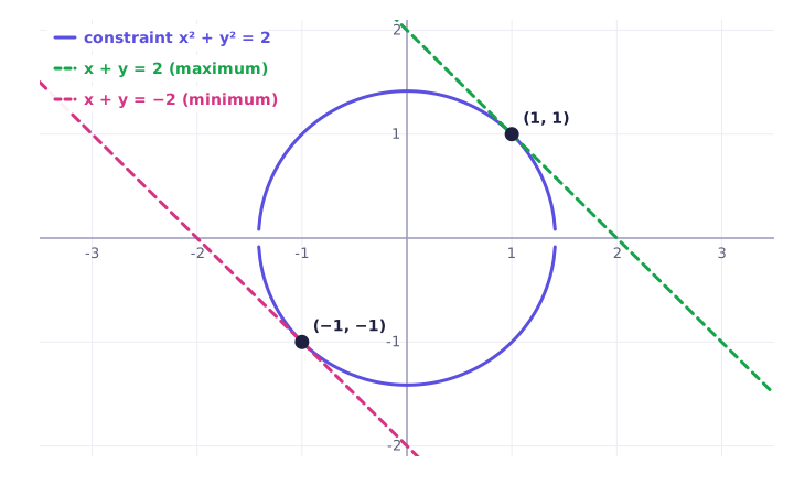
Find the maximum and minimum of f(x, y) = x + y on the circle x^2 + y^2 = 2.
Step 1. Gradients. \nabla f = \langle 1, 1 \rangle and, with g = x^2 + y^2, \nabla g = \langle 2x, 2y \rangle.
Step 2. The system.
Step 3. Eliminate \lambda. Neither \lambda, x nor y can be 0 (or 1 = 0). Solve for \lambda: \lambda = \frac{1}{2x} = \frac{1}{2y}, so x = y.
Step 4. Use the constraint. x^2 + x^2 = 2 gives x = \pm 1. The candidates are (1, 1) and (-1, -1).
Step 5. Evaluate. f(1, 1) = 2 and f(-1, -1) = -2.
The maximum is 2 at (1, 1) and the minimum is -2 at (-1, -1). In the graph, the level lines x + y = 2 and x + y = -2 just touch the circle, while any line in between, such as x + y = 0, cuts straight through it.
Worked example 2: a product on an ellipse
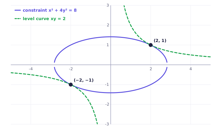
Find the maximum and minimum of f(x, y) = xy on the ellipse x^2 + 4y^2 = 8.
Step 1. Gradients. \nabla f = \langle y, x \rangle and \nabla g = \langle 2x, 8y \rangle.
Step 2. The system.
Step 3. Substitute. Put the second equation into the first: y = 2\lambda(8\lambda y) = 16\lambda^2 y, so y(1 - 16\lambda^2) = 0.
- Case y = 0. Then x = 8\lambda \cdot 0 = 0, but (0, 0) is not on the ellipse. No solution.
- Case \lambda^2 = \frac{1}{16}. Then \lambda = \pm\frac{1}{4}, and y = 2\lambda x = \pm\frac{x}{2}.
Step 4. Use the constraint. With y = \pm\frac{x}{2}, 4y^2 = x^2, so x^2 + x^2 = 8 and x = \pm 2. That gives four candidates: (2, 1), (-2, -1), (2, -1) and (-2, 1).
Step 5. Evaluate.
| Point | f = xy |
|---|---|
| (2, 1) | 2 |
| (-2, -1) | 2 |
| (2, -1) | -2 |
| (-2, 1) | -2 |
The maximum is 2, at (2, 1) and (-2, -1). The minimum is -2, at (2, -1) and (-2, 1). Since the ellipse is closed and bounded, both are guaranteed to exist.
The level curves of xy are hyperbolas. The hyperbola xy = 2 is tangent to the ellipse at the two maximum points, exactly as the parallel gradient condition predicts.
Worked example 3: closest point on a plane
Find the point on the plane x + 2y + 2z = 9 closest to the origin.
Step 1. Choose f. Distance is \sqrt{x^2 + y^2 + z^2}. Minimizing the square root is the same as minimizing what is inside, so use f = x^2 + y^2 + z^2. The constraint is g = x + 2y + 2z = 9.
Step 2. Gradients. \nabla f = \langle 2x, 2y, 2z \rangle and \nabla g = \langle 1, 2, 2 \rangle.
Step 3. The system.
Step 4. Express everything in terms of \lambda. x = \frac{\lambda}{2}, y = \lambda, z = \lambda.
Step 5. Use the constraint.
So the point is (1, 2, 2), and f = 1 + 4 + 4 = 9, giving a distance of \sqrt{9} = 3.
Step 6. Is it a min or a max? There is only one candidate, and a plane has points as far from the origin as you like, so there is no maximum. The single candidate must be the minimum. As a check, the point-to-plane distance formula gives \frac{|9|}{\sqrt{1 + 4 + 4}} = 3.
What does lambda mean?
The multiplier is not just a helper variable. \lambda is the rate at which the optimal value changes as the constraint constant c changes.
Check it on example 1 with a general circle x^2 + y^2 = c. The same steps give a maximum at x = y = \sqrt{c/2}, with value f^* = 2\sqrt{c/2} = \sqrt{2c}. Then
And at (1, 1), the equation 1 = 2\lambda x gave \lambda = \frac{1}{2}. They match. In economics this is the shadow price: how much more profit one extra unit of a limited resource is worth.
Common mistakes with Lagrange multipliers
- Dividing by a variable that could be zero. In example 2, dividing y = 16\lambda^2 y by y would hide the case y = 0. Factor instead, and handle each case.
- Forgetting the constraint equation. \nabla f = \lambda\nabla g alone has too many solutions. You need g = c to pin them down.
- Stopping before evaluating f. The system gives candidates, not answers.
- Missing sign cases. Square roots give \pm. Example 2 has four candidates, not one.
- Claiming a max that does not exist. On an unbounded constraint like a line or a plane, one of the extremes may not exist. Argue which one you found.
- Optimizing distance with the square root. It works, but the algebra is much cleaner with distance squared.
Quick reference: Lagrange multipliers
| Item | Two variables | Three variables |
|---|---|---|
| Goal | optimize f(x, y) with g(x, y) = c | optimize f(x, y, z) with g(x, y, z) = c |
| Equations | f_x = \lambda g_x, f_y = \lambda g_y, g = c | add f_z = \lambda g_z |
| Unknowns | x, y, \lambda | x, y, z, \lambda |
| Geometry | level curve of f tangent to the constraint | level surface of f tangent to the constraint |
| Deciding max or min | compare f at every candidate | compare f at every candidate |
Practice the algebra, master the method
The calculus in a Lagrange problem takes one line. The real work is solving the system without losing a case, and that only gets reliable with practice. The interactive lesson below gives you constrained problems to solve step by step, checks your system and each candidate point instantly, and shows you any case you missed.
Practice it now
Lagrange multipliers
Solve real problems on this topic with instant feedback, hints and a step-by-step walkthrough for every answer. Free, no sign-up needed to start.
Practice this lesson