Linear Approximation: Tangent Line Estimates and Differentials
Learn linear approximation step by step: the tangent line formula, estimating square roots like sqrt(4.1), differentials, error and over or underestimates.
By the PracticeCalculus team Published 7 min read
On this page
- What is linear approximation?
- Why the tangent line is a good estimate
- How to do a linear approximation in 4 steps
- Worked example 1: estimate the square root of 4.1
- Worked example 2: estimate the cube root of 27.3
- Worked example 3: estimate sin(0.1) and e^0.1
- Overestimate or underestimate? Use concavity
- Differentials: the same idea in different notation
- Worked example 4: error in the volume of a sphere
- Worked example 5: comparing dy with the true change
- Quick reference: common linear approximations near 0
- Common linear approximation mistakes
- Why linear approximation matters
- Practice estimating with tangent lines
You need \sqrt{4.1}, \sin(0.1) or the volume error in a measured sphere, and you do not have a calculator (or your exam does not allow one). Linear approximation turns these into one line of arithmetic by using the tangent line in place of the curve. It is also the idea behind error estimates in physics and engineering.
What is linear approximation?
Zoom in far enough on any smooth curve and it starts to look like a straight line. That straight line is the tangent line. Linear approximation means using the tangent line at a point a to estimate the function's value at nearby points.
The tangent line at x = a is called the linearization of f at a:
and for x close to a,
Read the formula as: start at the known height f(a), then move along the tangent with slope f'(a) for a horizontal distance of x - a.
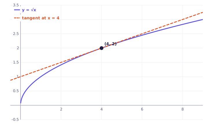
Notice that the tangent line sits slightly above the curve on both sides. That detail tells you whether your estimate is too big or too small, which we come back to below.
Why the tangent line is a good estimate
The derivative is defined as a limit of difference quotients:
So when x is close to a, the quotient \frac{f(x) - f(a)}{x - a} is close to f'(a). Multiply both sides by (x - a) and add f(a), and you get exactly f(x) \approx f(a) + f'(a)(x - a). Linear approximation is just the definition of the derivative, read backwards. This property of smooth functions, looking straight up close, is called local linearity.
It also explains why the estimate gets worse as you move away from a: the difference quotient drifts further from f'(a), and the curve bends away from the line.
How to do a linear approximation in 4 steps
- Choose f. Decide what function the number comes from, for example f(x) = \sqrt{x} for \sqrt{4.1}.
- Choose a nearby a where f(a) is easy to compute exactly. For square roots pick a perfect square, for trig pick an angle like 0 or \frac{\pi}{6}.
- Compute f(a) and f'(a) and write L(x).
- Plug in the value you want.
The whole skill is step 2. A good choice of a makes the arithmetic trivial and keeps the error small.
Worked example 1: estimate the square root of 4.1
Step 1. Let f(x) = \sqrt{x}. Then f'(x) = \frac{1}{2\sqrt{x}}.
Step 2. The closest perfect square to 4.1 is 4, so a = 4.
Step 3. f(4) = 2 and f'(4) = \frac{1}{2 \cdot 2} = \frac{1}{4}. So
Step 4. Plug in x = 4.1:
The true value is \sqrt{4.1} = 2.024846\ldots, so the estimate is off by about 0.00015. Not bad for mental math.
Worked example 2: estimate the cube root of 27.3
Step 1. Let f(x) = x^{1/3}, so f'(x) = \frac{1}{3}x^{-2/3}.
Step 2. 27 is a perfect cube near 27.3, so a = 27.
Step 3. f(27) = 3. For the slope, 27^{2/3} = 9, so f'(27) = \frac{1}{3 \cdot 9} = \frac{1}{27}. The linearization is
Step 4.
The true value is about 3.01109. The estimate is correct to four decimal places.
Worked example 3: estimate sin(0.1) and e^0.1
For f(x) = \sin x at a = 0: f(0) = 0 and f'(0) = \cos 0 = 1, so L(x) = x. Therefore
The true value is 0.09983\ldots This is the famous small angle approximation \sin x \approx x (with x in radians), used everywhere in physics, for example for a swinging pendulum.
For f(x) = e^x at a = 0: f(0) = 1 and f'(0) = 1, so L(x) = 1 + x and
compared with the true 1.10517\ldots
Overestimate or underestimate? Use concavity
The second derivative tells you which side of the curve the tangent line is on:
- If f''(a) < 0 (concave down), the curve bends below the tangent, so L(x) is an overestimate.
- If f''(a) > 0 (concave up), the curve bends above the tangent, so L(x) is an underestimate.
Check example 1: f''(x) = -\frac{1}{4}x^{-3/2}, which is negative at x = 4. So 2.025 should be too big, and it is (2.025 > 2.02485). For e^x, the second derivative is e^x > 0, so 1.1 is too small, which matches 1.1 < 1.10517.
Tip: exam questions love asking "is your estimate an over or underestimate, and why?" The answer is always about the sign of f'' near a.
Differentials: the same idea in different notation
Write dx for a small change in x. The differential dy is the change in height along the tangent line:
The true change in the function is \Delta y = f(x + dx) - f(x). Linear approximation says that for small dx,
This is exactly the linearization rearranged: f(a + dx) \approx f(a) + f'(a)\,dx. Differentials are most useful when the question is about a change or an error, rather than a value.
Worked example 4: error in the volume of a sphere
A sphere's radius is measured as 10 cm, with a possible error of \pm 0.1 cm. Estimate the maximum error in the computed volume.
Step 1. Write the formula. V = \frac{4}{3}\pi r^3.
Step 2. Take the differential. dV = 4\pi r^2\,dr.
Step 3. Plug in r = 10 and dr = 0.1:
Step 4. Relative error. The volume is V = \frac{4}{3}\pi(1000) \approx 4188.8 cm³, so
A 1\% error in the radius becomes about a 3\% error in the volume. The factor 3 comes from the exponent in r^3, a pattern worth remembering.
Worked example 5: comparing dy with the true change
A square has side s = 5 cm. Use differentials to estimate how much its area grows when the side increases to 5.02 cm, and compare with the exact change.
Step 1. A = s^2, so dA = 2s\,ds.
Step 2. With s = 5 and ds = 0.02: dA = 2(5)(0.02) = 0.2 cm².
Step 3. Exact change. \Delta A = (5.02)^2 - 5^2 = 25.2004 - 25 = 0.2004 cm².
The differential misses only the tiny corner square (ds)^2 = 0.0004. Picture the square growing: two thin strips of area s\,ds each make up dA, and the little corner piece is what the linear estimate ignores. That leftover is always about the size of (ds)^2, which is why the approximation is so good for small changes.
Quick reference: common linear approximations near 0
All of these come from L(x) = f(0) + f'(0)x and work best for small x:
| Function | Linear approximation near x = 0 |
|---|---|
| \sin x | x |
| \tan x | x |
| \cos x | 1 |
| e^x | 1 + x |
| \ln(1 + x) | x |
| (1 + x)^k | 1 + kx |
| \sqrt{1+x} | 1 + \frac{x}{2} |
The last two are the same rule. For example (1.02)^{10} \approx 1 + 10(0.02) = 1.2, close to the true 1.219.
Common linear approximation mistakes
- Choosing a badly. Using a = 0 for \sqrt{4.1} fails, since \sqrt{x} is not even differentiable at 0. Always pick a nearby point where the values are exact.
- Plugging x into the slope. The slope is the number f'(a), not the function f'(x). In example 1 the slope is \frac{1}{4}, full stop.
- Forgetting the (x - a). Writing L(4.1) = 2 + \frac{1}{4}(4.1) gives nonsense. You multiply the slope by the distance from a, which is 0.1.
- Using degrees with trig. \sin x \approx x only works in radians. \sin(5^\circ) is about 0.087, not 5.
- Trusting it far from a. The tangent line drifts away from the curve as you move away from a. \sqrt{9} \approx L(9) = 3.25 is noticeably wrong.
Why linear approximation matters
Linear approximation is more than a trick for square roots. It is the reason calculators, physics formulas and numerical methods work: Newton's method repeatedly uses tangent lines to solve equations, and Taylor polynomials (see Taylor series) extend the idea from lines to parabolas and beyond. It also connects to the mean value theorem, which guarantees that some tangent line matches the average slope exactly.
Practice estimating with tangent lines
The steps are always the same: pick f, pick a friendly a, find f(a) and f'(a), then plug in. A dozen practice problems is usually enough for it to become automatic. The interactive lesson below gives you instant feedback on each estimate and shows exactly where a slope or a distance went wrong.
Practice it now
Tangent lines at work
Solve real problems on this topic with instant feedback, hints and a step-by-step walkthrough for every answer. Free, no sign-up needed to start.
Practice this lesson