Properties of Definite Integrals: Rules, Symmetry and Examples
The properties of definite integrals: reversing limits, zero width, additivity over intervals, odd and even symmetry and comparison bounds, with examples.
Integration rules Updated 3 min read
At a glance
- Zero width
- \int_a^a f(x)\,dx = 0
- Reversed limits
- \int_b^a f(x)\,dx = -\int_a^b f(x)\,dx
- Constant
- \int_a^b k\,dx = k(b - a)
- Odd function
- \int_{-a}^{a} f(x)\,dx = 0
- Even function
- \int_{-a}^{a} f(x)\,dx = 2\int_0^a f(x)\,dx
- Comparison
- If f(x) \le g(x) on [a, b], then \int_a^b f\,dx \le \int_a^b g\,dx
On this page
The properties of definite integrals are the rules for manipulating \int_a^b f(x)\,dx without computing it from scratch: flipping limits, splitting intervals, using symmetry and estimating size. They all follow from viewing the integral as signed area, or from the Fundamental Theorem of Calculus.
The properties
Assume f and g are integrable on the intervals involved.
| Property | Statement |
|---|---|
| Zero width | \int_a^a f(x)\,dx = 0 |
| Reversed limits | \int_b^a f(x)\,dx = -\int_a^b f(x)\,dx |
| Constant | \int_a^b k\,dx = k(b-a) |
| Linearity | \int_a^b [\alpha f + \beta g]\,dx = \alpha\int_a^b f\,dx + \beta\int_a^b g\,dx |
| Additivity | \int_a^b f\,dx + \int_b^c f\,dx = \int_a^c f\,dx |
| Comparison | f \le g on [a,b] \Rightarrow \int_a^b f\,dx \le \int_a^b g\,dx |
| Bounds | m \le f \le M on [a,b] \Rightarrow m(b-a) \le \int_a^b f\,dx \le M(b-a) |
| Odd symmetry | f(-x) = -f(x) \Rightarrow \int_{-a}^{a} f\,dx = 0 |
| Even symmetry | f(-x) = f(x) \Rightarrow \int_{-a}^{a} f\,dx = 2\int_0^a f\,dx |
The comparison and bounds properties assume a < b. Additivity holds for any order of a, b and c, as long as f is integrable on the intervals, thanks to the reversed-limits rule.
Why they hold
If F is an antiderivative of f, then \int_a^b f\,dx = F(b) - F(a). Each property is a line of algebra from there:
- zero width: F(a) - F(a) = 0;
- reversed limits: F(a) - F(b) = -\left(F(b) - F(a)\right);
- additivity: \left(F(b) - F(a)\right) + \left(F(c) - F(b)\right) = F(c) - F(a).
Linearity is covered on its own page: integral linearity rules.
Symmetry: odd and even functions
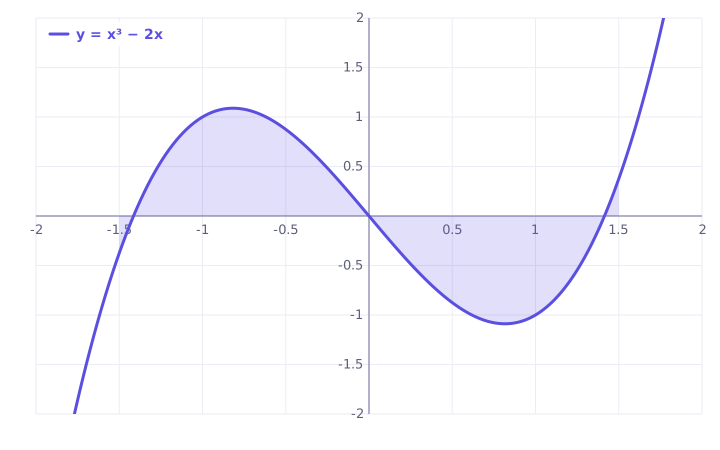
An odd function is symmetric about the origin, so every bit of positive area has a matching bit of negative area. An even function is symmetric about the y-axis, so the two halves are equal and you can double one of them. Checking symmetry first can turn a long calculation into one line.
Worked examples
Example 1: odd symmetry. x^5 - 4x^3 + \sin x is odd, so
Example 2: even symmetry. x^2 is even, so
Example 3: additivity and reversed limits. Given \int_0^5 f(x)\,dx = 10 and \int_0^2 f(x)\,dx = 3:
Example 4: an absolute value. Split where the inside changes sign. On [-1, 0], \lvert x\rvert = -x; on [0, 2], \lvert x\rvert = x:
Example 5: estimating with bounds. On [0, 1], e^{-1} \le e^{-x^2} \le 1, so
This integral has no elementary antiderivative, yet the bounds pin it down. Its actual value is about 0.747.
Common mistakes
- Using symmetry on a non-symmetric interval. \int_{-1}^{2} x^3\,dx is not 0. The interval must be [-a, a].
- Calling a function odd without checking. x^3 + 1 is neither odd nor even, so \int_{-1}^{1} (x^3 + 1)\,dx = 2, not 0.
- Forgetting the sign flip when reversing limits.
- Confusing signed area with total area. \int_{-1}^{1} x\,dx = 0, but the total shaded area is 1. For area, integrate \lvert f(x)\rvert, as in area between curves.
For how these properties connect to Riemann sums and evaluating integrals, see the guides to Riemann sums and the Fundamental Theorem of Calculus.
Practice it now
The definite integral as area
Solve real problems on this topic with instant feedback, hints and a step-by-step walkthrough for every answer. Free, no sign-up needed to start.
Practice this lesson