Mean Value Theorem for Integrals: Statement and Examples

The mean value theorem for integrals says a continuous function hits its own average value at least once. If you flatten the area under the curve into a rectangle of the same width, the rectangle's height is a value the function actually takes.

Statement of the mean value theorem for integrals

If f is continuous on the closed interval [a, b], then there exists a number c in [a, b] such that

or equivalently

The quantity on the right of the first equation is the average value of f on [a, b], written f_{\text{avg}}.

What the theorem means

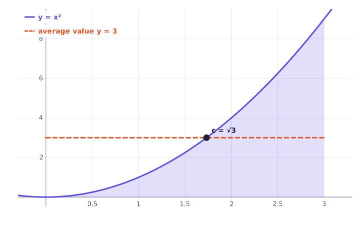
The area under y = f(x) from a to b equals the area of a rectangle with the same base, b - a, and height f_{\text{avg}}. The theorem says that height is not just some number: the curve passes through it. Picture water in a tank with a wavy surface. When the water settles flat, its level is the average height, and the original wavy surface was at that level somewhere.

Why continuity matters

Let f(x) = 0 for 0 \le x < 1 and f(x) = 1 for 1 \le x \le 2. Its integral over [0, 2] is 1, so its average value is \frac{1}{2}. But f only takes the values 0 and 1, never \frac{1}{2}. The jump at x = 1 lets the function skip over its average. With continuity, the intermediate value theorem rules this out.

Why the theorem is true

By the extreme value theorem, f has a minimum m and maximum M on [a, b]. Since m \le f(x) \le M,

So f_{\text{avg}} lies between two values that f attains, and the intermediate value theorem gives a c with f(c) = f_{\text{avg}}.

Worked examples

Example 1: f(x) = x^2 on [0, 3].

Step 1. Average value: \frac{1}{3 - 0}\int_0^3 x^2\,dx = \frac{1}{3}\left[\frac{x^3}{3}\right]_0^3 = \frac{1}{3}\cdot 9 = 3.

Step 2. Solve c^2 = 3, so c = \pm\sqrt{3}.

Step 3. Only c = \sqrt{3} \approx 1.732 lies in [0, 3].

Example 2: f(x) = \sin x on [0, \pi].

Step 1. f_{\text{avg}} = \frac{1}{\pi}\int_0^\pi \sin x\,dx = \frac{1}{\pi}\cdot 2 = \frac{2}{\pi} \approx 0.637.

Step 2. Solve \sin c = \frac{2}{\pi}. On [0, \pi] there are two solutions:

The theorem promises at least one; here there are two.

Example 3: a linear function. For f(x) = 2x + 1 on [0, 4], \int_0^4 (2x + 1)\,dx = \big[x^2 + x\big]_0^4 = 20, so f_{\text{avg}} = \frac{20}{4} = 5. Solving 2c + 1 = 5 gives c = 2, the midpoint. For any linear function the average value is reached at the midpoint.

Common mistakes

1. Forgetting to divide by b - a. The integral is the area; the average value is the area divided by the width.
2. Keeping solutions outside the interval. In Example 1, c = -\sqrt{3} must be discarded.
3. Confusing it with the MVT for derivatives. That theorem matches f'(c) to the average slope of f. This one matches f(c) to the average value of f.

Related theorems

This theorem is the mean value theorem applied to F(x) = \int_a^x f(t)\,dt, using FTC part 1 for F' = f and FTC part 2 to evaluate the integral. For more on integrals as accumulated area, see Riemann sums and the fundamental theorem of calculus guide.