Intermediate Value Theorem (IVT): Statement and Examples

The intermediate value theorem (IVT) says that a continuous function cannot skip values. If it starts at one height and ends at another, it must pass through every height in between. It is the standard way to prove that an equation has a solution without solving it.

Statement of the intermediate value theorem

Suppose that

1. f is continuous on the closed interval [a, b], and
2. N is any number strictly between f(a) and f(b).

Then there exists at least one number c in the open interval (a, b) such that

The most common special case is about roots: if f is continuous on [a, b] and f(a) and f(b) have opposite signs, then f(c) = 0 for some c in (a, b). This version is sometimes called Bolzano's theorem.

What the IVT means

Draw a continuous curve from the point (a, f(a)) to the point (b, f(b)) without lifting your pencil. Any horizontal line y = N between the two heights has to be crossed. The IVT is the precise version of that drawing.

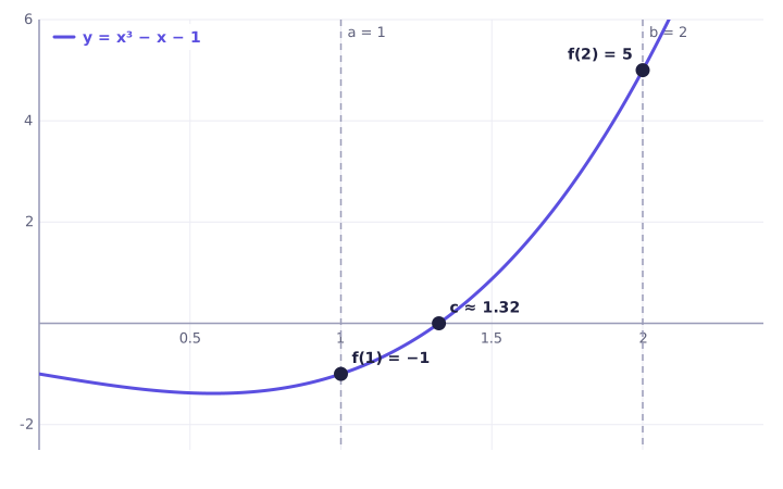
Notice what the theorem does not say. It does not say where c is, and it does not say c is unique. It is an existence theorem.

Why continuity matters: counterexamples

A vertical asymptote. Let f(x) = \frac{1}{x} on [-1, 1]. Then f(-1) = -1 and f(1) = 1, so 0 is between them, yet \frac{1}{x} is never 0. The IVT does not apply because f is not defined, let alone continuous, at x = 0.

A jump. Let f(x) = 0 for x < 1 and f(x) = 2 for x \ge 1, on [0, 2]. The function goes from 0 to 2 but never equals 1. The jump at x = 1 breaks continuity.

Continuity on part of the interval is not enough. The hypothesis is continuity on all of [a, b], including the endpoints. Checking a few points proves nothing. See the guide on continuity for how to check it.

Worked examples

Example 1: show x^3 - x - 1 = 0 has a solution between 1 and 2.

Step 1. f(x) = x^3 - x - 1 is a polynomial, so it is continuous on [1, 2].

Step 2. f(1) = 1 - 1 - 1 = -1 and f(2) = 8 - 2 - 1 = 5.

Step 3. Since -1 < 0 < 5, the IVT gives a c in (1, 2) with f(c) = 0.

Step 4 (narrowing it down). f(1.5) = 3.375 - 1.5 - 1 = 0.875 > 0, so the sign change, and therefore a root, is in (1, 1.5). Repeating this halving is the bisection method, which pins the root down to c \approx 1.3247.

Example 2: show \cos x = x has a solution.

Move everything to one side: g(x) = \cos x - x, which is continuous everywhere. Then

By the IVT, g(c) = 0 for some c in (0, \frac{\pi}{2}), so \cos c = c. You could never solve this equation with algebra, but the IVT proves the solution exists.

Example 3: hitting a value other than zero. Show that f(x) = x^2 + x takes the value 4 on [1, 2]. f is continuous, f(1) = 2 and f(2) = 6. Since 2 < 4 < 6, there is a c in (1, 2) with c^2 + c = 4. (Solving gives c = \frac{-1 + \sqrt{17}}{2} \approx 1.56, which is indeed in the interval.)

How to write an IVT argument

A complete answer on an exam names all three pieces:

1. Continuity: state why f is continuous on [a, b] (polynomial, sum of continuous functions, and so on).
2. Endpoint values: compute f(a) and f(b).
3. Conclusion: say that N lies between them, so by the intermediate value theorem some c in (a, b) has f(c) = N.

Common mistakes

1. Skipping the continuity check. Without it the argument is incomplete, and for functions like \tan x or \frac{1}{x} the conclusion can be false.
2. Claiming exactly one solution. The IVT gives at least one. Uniqueness needs a separate argument, for example that f is strictly increasing.
3. Using the converse. A function that takes every intermediate value is not necessarily continuous. The IVT only runs one way.

Related theorems

The IVT is a companion to the extreme value theorem: both rely on continuity on a closed interval. To prove a root is the only one, pair the IVT with Rolle's theorem. For limit techniques behind continuity, see how to evaluate limits and the squeeze theorem.