Riemann Sums: Left, Right and Midpoint Rules With Examples
Learn Riemann sums step by step: left, right and midpoint rectangles, sigma notation, over and underestimates, and how the limit becomes the definite integral.
By the PracticeCalculus team Published 7 min read
On this page
- What is a Riemann sum?
- Left, right and midpoint Riemann sums
- Worked example 1: area under y = x² from 0 to 2
- Overestimate or underestimate?
- Worked example 2: a decreasing function
- Worked example 3: Riemann sums from a table
- Writing Riemann sums in sigma notation
- From Riemann sums to the definite integral
- Common Riemann sum mistakes
- Practice with rectangles
Finding the area of a rectangle is easy. Finding the area under a curve like y = x^2 is not, because the top edge bends. Riemann sums solve this by filling the region with thin rectangles and adding them up, and they are the idea that the entire definite integral is built on.
What is a Riemann sum?
A Riemann sum is an estimate of the area under y = f(x) on an interval [a, b] made of rectangles:
- Split [a, b] into n equal pieces, each of width
- In each piece, pick a sample point x_i^* and use f(x_i^*) as the rectangle's height.
- Add up the areas, height times width:
The only choice you make is where in each piece to take the height. That choice gives the three standard rules.
Left, right and midpoint Riemann sums
With x_0 = a, x_1 = a + \Delta x, x_2 = a + 2\Delta x, and so on up to x_n = b:
| Rule | Sample point in piece i | Sum |
|---|---|---|
| Left sum | left end, x_{i-1} = a + (i-1)\Delta x | L_n = \Delta x\,[f(x_0) + f(x_1) + \cdots + f(x_{n-1})] |
| Right sum | right end, x_i = a + i\,\Delta x | R_n = \Delta x\,[f(x_1) + f(x_2) + \cdots + f(x_n)] |
| Midpoint sum | middle, a + (i - \frac{1}{2})\Delta x | M_n = \Delta x\,[f(m_1) + f(m_2) + \cdots + f(m_n)] |
Notice that the left sum uses every point except the last, and the right sum uses every point except the first.
Worked example 1: area under y = x² from 0 to 2
Estimate \int_0^2 x^2\,dx with n = 4 using left, right and midpoint sums.
Step 1. Width. \Delta x = \frac{2 - 0}{4} = 0.5. The division points are 0, 0.5, 1, 1.5, 2.
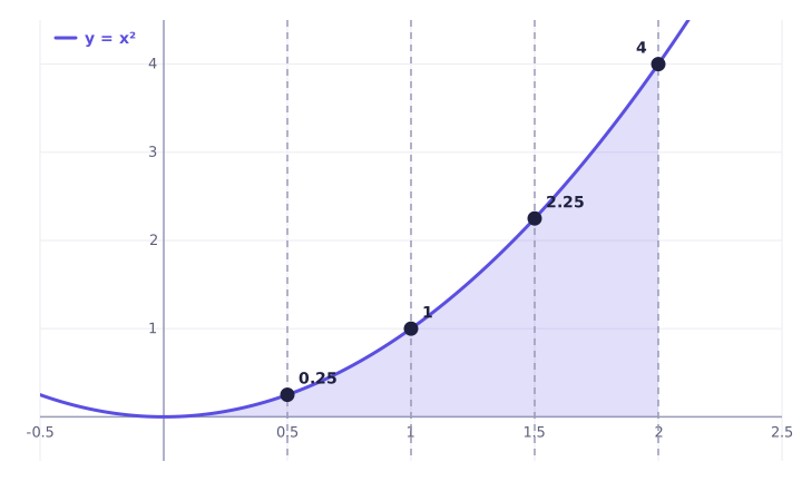
Step 2. Left sum. Heights at 0, 0.5, 1, 1.5:
Step 3. Right sum. Heights at 0.5, 1, 1.5, 2:
Step 4. Midpoint sum. Midpoints 0.25, 0.75, 1.25, 1.75:
The exact area (which we will confirm below) is \frac{8}{3} \approx 2.667. The left sum is far too low, the right sum far too high, and the midpoint sum is off by only 0.04.
Overestimate or underestimate?
On an increasing function like x^2 on [0, 2], the left end of each piece is the lowest point, so every left rectangle sits under the curve: left sums underestimate. The right end is the highest point, so right sums overestimate. For a decreasing function, swap the two.
The midpoint rule depends on concavity instead. On a concave up curve like x^2, the midpoint sum underestimates (just slightly), and on a concave down curve it overestimates.
| Function shape | Left sum | Right sum | Midpoint sum |
|---|---|---|---|
| Increasing | Under | Over | (check concavity) |
| Decreasing | Over | Under | (check concavity) |
| Concave up | Under | ||
| Concave down | Over |
Averaging the left and right sums gives the trapezoid rule: \frac{1.75 + 3.75}{2} = 2.75. On a concave up curve the trapezoid rule overestimates, so the true value sits between the midpoint and trapezoid estimates: 2.625 < \frac{8}{3} < 2.75.
Worked example 2: a decreasing function
Estimate \int_1^3 \frac{1}{x}\,dx with n = 4 using all three rules.
Step 1. Width. \Delta x = \frac{3 - 1}{4} = 0.5. Division points: 1, 1.5, 2, 2.5, 3.
Step 2. Left sum. Heights f(1) = 1, f(1.5) \approx 0.6667, f(2) = 0.5, f(2.5) = 0.4:
Step 3. Right sum. Heights at 1.5, 2, 2.5, 3:
Step 4. Midpoint sum. Midpoints 1.25, 1.75, 2.25, 2.75 give heights 0.8, 0.5714, 0.4444, 0.3636:
The exact value is \ln 3 \approx 1.0986. This time the function is decreasing, so the left sum is too big and the right sum is too small: the opposite of example 1. The curve is concave up, so the midpoint sum is again slightly low.
Worked example 3: Riemann sums from a table
A car's velocity is recorded every second:
| t (s) | 0 | 1 | 2 | 3 | 4 |
|---|---|---|---|---|---|
| v (m/s) | 0 | 4 | 7 | 9 | 10 |
Estimate the distance traveled from t = 0 to t = 4.
Distance is the area under the velocity curve, and \Delta t = 1.
Left sum: 1 \cdot (0 + 4 + 7 + 9) = 20 m.
Right sum: 1 \cdot (4 + 7 + 9 + 10) = 30 m.
The velocity only increases in the table, so (assuming it increases between readings too) the true distance is between 20 and 30 meters. You cannot use a midpoint sum with n = 4 here, because the table has no readings at t = 0.5, 1.5, \ldots. With n = 2 you could: midpoints t = 1 and t = 3 give 2 \cdot (4 + 9) = 26 m.
Writing Riemann sums in sigma notation
For a right sum on [a, b] with n pieces, the sample points are x_i = a + i\,\Delta x, so
For left sums replace i with i - 1; for midpoints replace it with i - \frac{1}{2}.
Worked example 4: the exact area as a limit
Find \int_0^2 x^2\,dx as the limit of right sums.
Step 1. Set up. \Delta x = \frac{2}{n} and x_i = \frac{2i}{n}, so f(x_i) = \frac{4i^2}{n^2}.
Step 2. Write the sum.
Step 3. Use the sum of squares formula \sum_{i=1}^{n} i^2 = \frac{n(n+1)(2n+1)}{6}:
Step 4. Take the limit. As n \to \infty, both \frac{1}{n} terms go to 0:
So the exact area is \frac{8}{3}. With n = 4 the formula gives \frac{4}{3}(1.25)(2.25) = 3.75, matching worked example 1.
From Riemann sums to the definite integral
The calculation above is exactly how the definite integral is defined:
The notation even mirrors the sum: \int is a stretched "S" for sum, f(x) is the height, and dx is the infinitely thin width. Where f is negative, the rectangles have negative height, so the integral measures signed area: area above the axis counts as positive and area below as negative.
Computing a limit of sums every time would be painful. The fundamental theorem of calculus shows that you can skip it: \int_0^2 x^2\,dx = \left[\frac{x^3}{3}\right]_0^2 = \frac{8}{3}, using antiderivatives. Riemann sums are still how you approximate integrals from data or from functions with no simple antiderivative.
Common Riemann sum mistakes
- Using n + 1 heights. With n = 4 there are 5 division points but only 4 rectangles. A left sum drops the last point; a right sum drops the first.
- Forgetting to multiply by \Delta x. Adding the heights gives 7.5 in example 1, not the area 3.75.
- Wrong midpoints. The midpoint of [1, 1.5] is 1.25. Compute f(1.25), not the average of f(1) and f(1.5) (that is the trapezoid rule).
- Unequal widths from a table. If the data are not evenly spaced, each rectangle needs its own width. Do not use a single \Delta x.
- Mixing up over and under. Increasing or decreasing decides left and right sums; concavity decides the midpoint and trapezoid rules.
Practice with rectangles
Riemann sums reward a steady routine: find \Delta x, list the sample points, evaluate, add, multiply. The interactive lesson below lets you build left, right and midpoint sums with instant feedback, so you can see exactly which height or width went wrong and fix it on the next try.
Practice it now
Area with rectangles
Solve real problems on this topic with instant feedback, hints and a step-by-step walkthrough for every answer. Free, no sign-up needed to start.
Practice this lesson